author: zlotus

Description:

這是MIT 18.06 Linear-Algebra 的學習筆記

Course video

第十六講：投影矩陣和最小二乘

上一講中，我們知道了投影矩陣$P=A(A^TA)^{-1}A^T$，$Pb$將會把向量投影在$A$的行空間中。

舉兩個極端的例子：

• 如果$b\in C(A)$，則$Pb=b$；
• 如果$b\bot C(A)$，則$Pb=0$。

一般情況下，$b$將會有一個垂直於$A$的分量，有一個在$A$行空間中的分量，投影的作用就是去掉垂直分量而保留行空間中的分量。

在第一個極端情況中，如果$b\in C(A)$則有$b=Ax$。帶入投影矩陣$p=Pb=A(A^TA)^{-1}A^TAx=Ax$，得證。

在第二個極端情況中，如果$b\bot C(A)$則有$b\in N(A^T)$，即$A^Tb=0$。則$p=Pb=A(A^TA)^{-1}A^Tb=0$，得證。

向量$b$投影後，有$b=e+p, p=Pb, e=(I-P)b$，這里的$p$是$b$在$C(A)$中的分量，而$e$是$b$在$N(A^T)$中的分量。

回到上一講最後提到的例題：

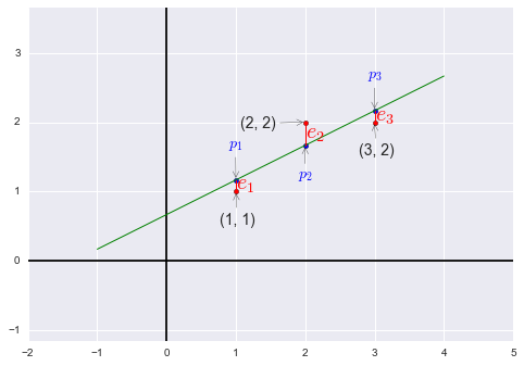
我們需要找到距離圖中三個點 $(1, 1), (2, 2), (3, 2)$ 偏差最小的直線：$y=C+Dt$。

%matplotlib inline
import matplotlib.pyplot as plt
from sklearn import linear_model
import numpy as np
import pandas as pd
import seaborn as sns

x = np.array([1, 2, 3]).reshape((-1,1))
y = np.array([1, 2, 2]).reshape((-1,1))
predict_line = np.array([-1, 4]).reshape((-1,1))

regr = linear_model.LinearRegression()
regr.fit(x, y)
ey = regr.predict(x)

fig = plt.figure()
plt.axis('equal')
plt.axhline(y=0, c='black')
plt.axvline(x=0, c='black')

plt.scatter(x, y, c='r')
plt.scatter(x, regr.predict(x), s=20, c='b')
plt.plot(predict_line, regr.predict(predict_line), c='g', lw='1')
[ plt.plot([x[i], x[i]], [y[i], ey[i]], 'r', lw='1') for i in range(len(x))]

plt.annotate('(1, 1)', xy=(1, 1), xytext=(-15, -30), textcoords='offset points', size=14, arrowprops=dict(arrowstyle="->"))
plt.annotate('(2, 2)', xy=(2, 2), xytext=(-60, -5), textcoords='offset points', size=14, arrowprops=dict(arrowstyle="->"))
plt.annotate('(3, 2)', xy=(3, 2), xytext=(-15, -30), textcoords='offset points', size=14, arrowprops=dict(arrowstyle="->"))

plt.annotate('$e_1$', color='r', xy=(1, 1), xytext=(0, 2), textcoords='offset points', size=20)
plt.annotate('$e_2$', color='r', xy=(2, 2), xytext=(0, -15), textcoords='offset points', size=20)
plt.annotate('$e_3$', color='r', xy=(3, 2), xytext=(0, 1), textcoords='offset points', size=20)

plt.annotate('$p_1$', xy=(1, 7/6), color='b', xytext=(-7, 30), textcoords='offset points', size=14, arrowprops=dict(arrowstyle="->"))
plt.annotate('$p_2$', xy=(2, 5/3), color='b', xytext=(-7, -30), textcoords='offset points', size=14, arrowprops=dict(arrowstyle="->"))
plt.annotate('$p_3$', xy=(3, 13/6), color='b', xytext=(-7, 30), textcoords='offset points', size=14, arrowprops=dict(arrowstyle="->"))
plt.draw()

plt.close(fig)

根據條件可以得到方程組 $ \begin{cases} C+D&=1 \
C+2D&=2 \
C+3D&=2 \
\end{cases} $，寫作矩陣形式 \(\begin{bmatrix}1&1 \\1&2 \\1&3\\\end{bmatrix}\begin{bmatrix}C\\D\\\end{bmatrix}=\begin{bmatrix}1\\2\\2\\\end{bmatrix}\)，也就是我們的$Ax=b$，很明顯方程組無解。

我們需要在$b$的三個分量上都增加某個誤差$e$，使得三點能夠共線，同時使得$e_1^2+e_2^2+e_3^2$最小，找到擁有最小平方和的解（即最小二乘），即$\left|Ax-b\right|^2=\left|e\right|^2$最小。此時向量$b$變為向量$p=\begin{bmatrix}p_1\\p_2\\p_3\end{bmatrix}$（在方程組有解的情況下，$Ax-b=0$，即$b$在$A$的行空間中，誤差$e$為零。）我們現在做的運算也稱作線性回歸（linear regression），使用誤差的平方和作為測量總誤差的標準。

注：如果有另一個點，如$(0, 100)$，在本例中該點明顯距離別的點很遠，最小二乘將很容易被離群的點影響，通常使用最小二乘時會去掉明顯離群的點。

現在我們嘗試解出$\hat x=\begin{bmatrix}\hat C\\ \hat D\end{bmatrix}$與$p=\begin{bmatrix}p_1\\p_2\\p_3\end{bmatrix}$。

寫作方程形式為$\begin{cases}3\hat C+16\hat D&=5\\6\hat C+14\hat D&=11\end{cases}$，也稱作正規方程組（normal equations）。

回顧前面提到的“使得誤差最小”的條件，$e_1^2+e_2^2+e_3^2=(C+D-1)^2+(C+2D-2)^2+(C+3D-2)^2$，使該式取最小值，如果使用微積分方法，則需要對該式的兩個變量$C, D$分別求偏導數，再令求得的偏導式為零即可，正是我們剛才求得的正規方程組。（正規方程組中的第一個方程是對$C$求偏導的結果，第二個方程式對$D$求偏導的結果，無論使用哪一種方法都會得到這個方程組。）

解方程得$\hat C=\frac{2}{3}, \hat D=\frac{1}{2}$，則“最佳直線”為$y=\frac{2}{3}+\frac{1}{2}t$，帶回原方程組解得$p_1=\frac{7}{6}, p_2=\frac{5}{3}, p_3=\frac{13}{6}$，即$e_1=-\frac{1}{6}, e_2=\frac{1}{3}, e_3=-\frac{1}{6}$

於是我們得到$p=\begin{bmatrix}\frac{7}{6}\\\frac{5}{3}\\\frac{13}{6}\end{bmatrix}, e=\begin{bmatrix}-\frac{1}{6}\\\frac{1}{3}\\-\frac{1}{6}\end{bmatrix}$，易看出$b=p+e$，同時我們发現$p\cdot e=0$即$p\bot e$。

誤差向量$e$不僅垂直於投影向量$p$，它同時垂直於行空間，如 $\begin{bmatrix}1\\1\\1\end{bmatrix}, \begin{bmatrix}1\\2\\3\end{bmatrix}$。

接下來我們觀察$A^TA$，如果$A$的各行線性無關，求證$A^TA$是可逆矩陣。

先假設$A^TAx=0$，兩邊同時乘以$x^T$有$x^TA^TAx=0$，即$(Ax)^T(Ax)=0$。一個矩陣乘其轉置結果為零，則這個矩陣也必須為零（$(Ax)^T(Ax)$相當於$Ax$長度的平方）。則$Ax=0$，結合題設中的“$A$的各行線性無關”，可知$x=0$，也就是$A^TA$的零空間中有且只有零向量，得證。

我們再來看一種線性無關的特殊情況：互相垂直的單位向量一定是線性無關的。

• 比如$\begin{bmatrix}1\\0\\0\end{bmatrix}\begin{bmatrix}0\\1\\0\end{bmatrix}\begin{bmatrix}0\\0\\1\end{bmatrix}$，這三個正交單位向量也稱作標準正交向量組（orthonormal vectors）。
• 另一個例子$\begin{bmatrix}\cos\theta\\\sin\theta\end{bmatrix}\begin{bmatrix}-\sin\theta\\\cos\theta\end{bmatrix}$

下一講研究標準正交向量組。