author: zlotus

Description:

這是MIT 18.06 Linear-Algebra 的學習筆記

Course video

第十五講：子空間投影

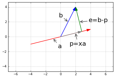
從$\mathbb{R}^2$空間講起，有向量$a, b$，做$b$在$a$上的投影$p$，如圖：

%matplotlib inline
import matplotlib.pyplot as plt
import numpy as np
import pandas as pd

plt.style.use("seaborn-dark-palette")

fig = plt.figure()
plt.axis('equal')
plt.axis([-7, 7, -6, 6])
plt.arrow(-4, -1, 8, 2, head_width=0.3, head_length=0.5, color='r', length_includes_head=True)
plt.arrow(0, 0, 2, 4, head_width=0.3, head_length=0.5, color='b', length_includes_head=True)
plt.arrow(0, 0, 48/17, 12/17, head_width=0.3, head_length=0.5, color='gray', length_includes_head=True)
plt.arrow(48/17, 12/17, 2-48/17, 4-12/17, head_width=0.3, head_length=0.5, color='g', length_includes_head=True)
# plt.plot([48/17], [12/17], 'o')
# y=1/4x
# y=-4x+12
# x=48/17
# y=12/17
plt.annotate('b', xy=(1, 2), xytext=(-30, 15), textcoords='offset points', size=20, arrowprops=dict(arrowstyle="->"))
plt.annotate('a', xy=(-1, -0.25), xytext=(15, -30), textcoords='offset points', size=20, arrowprops=dict(arrowstyle="->"))
plt.annotate('e=b-p', xy=(2.5, 2), xytext=(30, 0), textcoords='offset points', size=20, arrowprops=dict(arrowstyle="->"))
plt.annotate('p=xa', xy=(2, 0.5), xytext=(-20, -40), textcoords='offset points', size=20, arrowprops=dict(arrowstyle="->"))
plt.grid()

plt.close(fig)

從圖中我們知道，向量$e$就像是向量$b, p$之間的誤差，$e=b-p, e \bot p$。$p$在$a$上，有$\underline{p=ax}$。

所以有$a^Te=a^T(b-p)=a^T(b-ax)=0$。關於正交的最重要的方程：

從上面的式子可以看出，如果將$b$變為$2b$則$p$也會翻倍，如果將$a$變為$2a$則$p$不變。

設投影矩陣為$P$，則可以說投影矩陣作用與某個向量後，得到其投影向量，$projection_p=Pb$。

易看出$\underline{P=\frac{aa^T}{a^Ta}}$，若$a$是$n$維行向量，則$P$是一個$n \times n$矩陣。

觀察投影矩陣$P$的行空間，$C(P)$是一條通過$a$的直線，而$rank(P)=1$（一行乘以一列：$aa^T$，而這一行向量$a$是該矩陣的基）。

投影矩陣的性質：

• $\underline{P=P^T}$，投影矩陣是一個對稱矩陣。
• 如果對一個向量做兩次投影，即$PPb$，則其結果仍然與$Pb$相同，也就是$\underline{P^2=P}$。

為什麽我們需要投影？因為就像上一講中提到的，有些時候$Ax=b$無解，我們只能求出最接近的那個解。

$Ax$總是在$A$的行空間中，而$b$卻不一定，這是問題所在，所以我們可以將$b$變為$A$的行空間中最接近的那個向量，即將無解的$Ax=b$變為求有解的$A\hat{x}=p$（$p$是$b$在$A$的行空間中的投影，$\hat{x}$不再是那個不存在的$x$，而是最接近的解）。

現在來看$\mathbb{R}^3$中的情形，將向量$b$投影在平面$A$上。同樣的，$p$是向量$b$在平面$A$上的投影，$e$是垂直於平面$A$的向量，即$b$在平面$A$法方向的分量。 設平面$A$的一組基為$a_1, a_2$，則投影向量$p=\hat{x_1}a_1+\hat{x_2}a_2$，我們更傾向於寫作$p=A\hat{x}$，這里如果我們求出$\hat{x}$，則該解就是無解方程組最近似的解。

現在問題的關鍵在於找$e=b-A\hat{x}$，使它垂直於平面，因此我們得到兩個方程 $ \begin{cases}a_1^T(b-A\hat{x})=0\
a_2^T(b-A\hat{x})=0\end{cases} $，將方程組寫成矩陣形式 $ \begin{bmatrix}a_1^T\\a_2^T\end{bmatrix} (b-A\hat{x})= \begin{bmatrix}0\\0\end{bmatrix} $，即$A^T(b-A\hat{x})=0$。

比較該方程與$\mathbb{R}^2$中的投影方程，发現只是向量$a$變為矩陣$A$而已，本質上就是$A^Te=0$。所以，$e$在$A^T$的零空間中（$e\in N(A^T)$），從前面幾講我們知道，左零空間$\bot$行空間，則有$e\bot C(A)$，與我們設想的一致。

再化簡方程得$A^TAx=A^Tb$，比較在$\mathbb{R}^2$中的情形，$a^Ta$是一個數字而$A^TA$是一個$n$階方陣，而解出的$x$可以看做兩個數字的比值。現在在$\mathbb{R}^3$中，我們需要再次考慮：什麽是$\hat{x}$？投影是什麽？投影矩陣又是什麽？

• 第一個問題：$\hat x=(A^TA)^{-1}A^Tb$；
• 第二個問題：$p=A\hat x=\underline{A(A^TA)^{-1}A^T}b$，回憶在$\mathbb{R}^2$中的情形，下劃線部分就是原來的$\frac{aa^T}{a^Ta}$；
• 第三個問題：易看出投影矩陣就是下劃線部分$P=A(A^TA)^{-1}A^T$。

這里還需要注意一個問題，$P=A(A^TA)^{-1}A^T$是不能繼續化簡為$P=AA^{-1}(A^T)^{-1}A^T=I$的，因為這里的$A$並不是一個可逆方陣。 也可以換一種思路，如果$A$是一個$n$階可逆方陣，則$A$的行空間是整個$\mathbb{R}^n$空間，於是$b$在$\mathbb{R}^n$上的投影矩陣確實變為了$I$，因為$b$已經在空間中了，其投影不再改變。

再來看投影矩陣$P$的性質：

• $P=P^T$：有 $ \left[A(A^TA)^{-1}A^T\right]^T=A\left[(A^TA)^{-1}\right]^TA^T $，而$(A^TA)$是對稱的，所以其逆也是對稱的，所以有$A((A^TA)^{-1})^TA^T=A(A^TA)^{-1}A^T$，得證。
• $P^2=P$：有 $ \left[A(A^TA)^{-1}A^T\right]\left[A(A^TA)^{-1}A^T\right]=A(A^TA)^{-1}\left[(A^TA)(A^TA)^{-1}\right]A^T=A(A^TA)^{-1}A^T $，得證。

最小二乘法

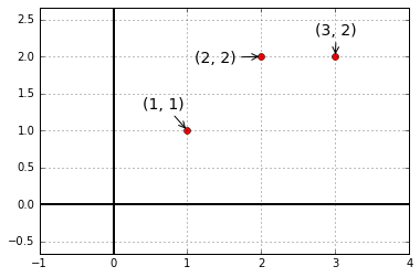
接下看看投影的經典應用案例：最小二乘法擬合直線（least squares fitting by a line）。

我們需要找到距離圖中三個點 $(1, 1), (2, 2), (3, 2)$ 偏差最小的直線：$b=C+Dt$。

plt.style.use("seaborn-dark-palette")

fig = plt.figure()
plt.axis('equal')
plt.axis([-1, 4, -1, 3])
plt.axhline(y=0, c='black', lw='2')
plt.axvline(x=0, c='black', lw='2')

plt.plot(1, 1, 'o', c='r')
plt.plot(2, 2, 'o', c='r')
plt.plot(3, 2, 'o', c='r')

plt.annotate('(1, 1)', xy=(1, 1), xytext=(-40, 20), textcoords='offset points', size=14, arrowprops=dict(arrowstyle="->"))
plt.annotate('(2, 2)', xy=(2, 2), xytext=(-60, -5), textcoords='offset points', size=14, arrowprops=dict(arrowstyle="->"))
plt.annotate('(3, 2)', xy=(3, 2), xytext=(-18, 20), textcoords='offset points', size=14, arrowprops=dict(arrowstyle="->"))

plt.grid()

plt.close(fig)

根據條件可以得到方程組 $ \begin{cases} C+D&=1 \
C+2D&=2 \
C+3D&=2 \
\end{cases} $，寫作矩陣形式 \(\begin{bmatrix}1&1 \\1&2 \\1&3\\\end{bmatrix}\begin{bmatrix}C\\D\\\end{bmatrix}=\begin{bmatrix}1\\2\\2\\\end{bmatrix}\)，也就是我們的$Ax=b$，很明顯方程組無解。但是$A^TA\hat x=A^Tb$有解，於是我們將原是兩邊同時乘以$A^T$後得到的新方程組是有解的，$A^TA\hat x=A^Tb$也是最小二乘法的核心方程。

下一講將進行最小二乘法的驗算。